Page 10 of 21

CM7.{5,8} | CM7.{5,8} | Study Designs, Association and Bias — SDL Guide

Learning Objectives

• Enumerate, define, describe, and discuss epidemiological study designs — descriptive and analytical (CM7.5)
• Describe the principles of association, causation, and biases in epidemiological studies (CM7.8)
• Calculate and interpret relative risk (RR) and odds ratio (OR) from 2×2 contingency tables
• Identify selection bias, information bias, and confounding in a study scenario and describe methods to control them

INSTRUCTIONS

How do we know that tobacco causes lung cancer — and not simply that lung cancer patients happen to smoke? How do we distinguish a genuine association from a spurious one produced by a flawed study design? Epidemiological study designs are the tools by which we translate observations into causal inferences — but only if the design is appropriate to the question and the analysis guards against systematic errors. This module builds the knowledge to read a study design diagram, calculate a measure of association, and identify the biases that may have invalidated the conclusions.

References

• Park's Textbook of Preventive and Social Medicine, 27th edition — Chapter 2: Epidemiology (Study Designs) (textbook)
• Gordis L. Epidemiology, 5th edition — Chapters 9–13: Cohort, Case-Control, and Experimental Studies (textbook)

---

Version 2.0 | NMC CBUC 2024

The Pyramid of Evidence: Why Study Design Determines Causal Confidence

Not all research designs are equal in their ability to establish causation. The hierarchy of evidence (evidence pyramid) ranks designs from lowest to highest causal confidence: case reports → case series → cross-sectional → ecological → case-control → cohort → randomised controlled trial (RCT) → systematic review + meta-analysis. The ranking reflects how well each design controls for confounding (the major threat to causal inference in observational studies) and establishes temporality (exposure must precede outcome).

The key features that determine causal confidence are:
1. Temporality: can the design establish that exposure preceded the disease? Cohort studies (prospective) establish this clearly; cross-sectional studies cannot, because exposure and outcome are measured simultaneously.
2. Comparison group: does the design include an unexposed or control group? Case reports describe only affected individuals; analytical designs (cohort, case-control) include a comparison group, enabling quantification of association.
3. Control of confounding: RCTs use randomisation; observational designs use restriction, matching, or statistical adjustment. The stronger the control, the more confident the causal inference.
4. Feasibility: RCTs are the gold standard but impossible for exposures that cannot be ethically randomised (tobacco, alcohol, radiation), rare outcomes (rare cancers), long latency periods (decades), or real-world generalisability. Observational designs fill this space.

For community medicine practice in India, the most commonly used designs are cross-sectional surveys (for burden estimation and programme planning) and case-control studies (for outbreak investigation and risk factor identification). Understanding when to use which design is the practical skill this module builds.

Descriptive Study Designs: Characterising Disease Distribution

Descriptive studies describe who gets disease, where, and when — without testing a causal hypothesis. They are hypothesis-generating, not hypothesis-testing.

Case reports describe a single patient with an unusual presentation, a novel diagnosis, or an unexpected drug reaction. They generate hypotheses for investigation but provide no comparison group and no population-level inference. The early AIDS cases in 1981 were first described as case reports of Pneumocystis pneumonia in young homosexual men — these reports triggered the cohort studies that identified the HIV virus.

Case series describe a group of patients sharing a common exposure or diagnosis — no comparison group, but patterns across cases can suggest aetiology. Thalidomide's teratogenicity was first suspected from a case series of infants with phocomelia (limb defects) born to women who had taken the drug.

Cross-sectional surveys (prevalence surveys) measure both exposure and outcome simultaneously in a defined population at a single point in time. They are efficient and relatively cheap; they measure prevalence (not incidence), so causation cannot be inferred (chicken-and-egg problem: does the exposure precede the disease, or does disease affect the exposure?). NFHS, NSS, and community health surveys are cross-sectional. Uses: estimating disease prevalence, assessing vaccination coverage, identifying disease distribution by person/place/time for programme planning.

Ecological studies use population-level (aggregate) data rather than individual-level data. They correlate disease rates with exposure rates across groups (countries, states, districts). For example, correlating per-capita salt intake by country with stroke mortality rates. The major limitation is the ecological fallacy (ecological correlation bias): a correlation at the group level does not imply the same association at the individual level — individuals within a high-salt country who have stroke may not be the same individuals with high salt intake.

Analytical Observational Designs: Cohort and Case-Control

Analytical designs include a comparison group and are designed to test a causal hypothesis — that an exposure is associated with an outcome.

Cohort study:
A group (cohort) of disease-free people is divided into those exposed and those unexposed to the factor of interest. They are followed forward in time until the outcome of interest occurs (or the study ends). Incidence rates are calculated in each group, and a Relative Risk (RR) is computed.

The 2×2 table for cohort studies:
``
Disease+ Disease-
Exposed: a b → a+b
Unexposed: c d → c+d
`

Relative Risk (RR) = Incidence in exposed / Incidence in unexposed = [a/(a+b)] / [c/(c+d)]

Interpretation: RR = 1.0 → no association; RR > 1.0 → exposure increases risk (risk factor); RR < 1.0 → exposure decreases risk (protective factor). RR = 3.0 means the exposed group has 3 times the risk of disease compared to the unexposed group.

Strengths: establishes temporality (exposure precedes outcome); can compute incidence and RR directly; can study multiple outcomes from a single exposure; reduces recall bias (exposure measured before disease). Limitations: expensive, time-consuming (especially for rare diseases with long latency); large sample required; losses to follow-up can bias results.

A retrospective cohort uses historical records to reconstruct the cohort — e.g. a company's employment records to trace occupational exposures, then linking to mortality records. It is logistically faster than a prospective cohort but limited by the quality of historical records.

Case-control study:
Cases (persons with the disease of interest) and controls (persons without the disease) are selected, then their past exposure histories are compared. The investigator starts at the outcome and looks backward.

The 2×2 table for case-control studies:
`
Cases Controls
Exposed: a b
Unexposed: c d
``

Odds Ratio (OR) = (Odds of exposure in cases) / (Odds of exposure in controls) = (a/c) / (b/d) = ad/bc

The OR cannot be interpreted as a direct risk estimate (because cases and controls are selected in a fixed ratio, not sampled from the population at their natural frequency). However, when the disease is rare (incidence <5–10%), the OR approximates the RR — this is the rare disease assumption.

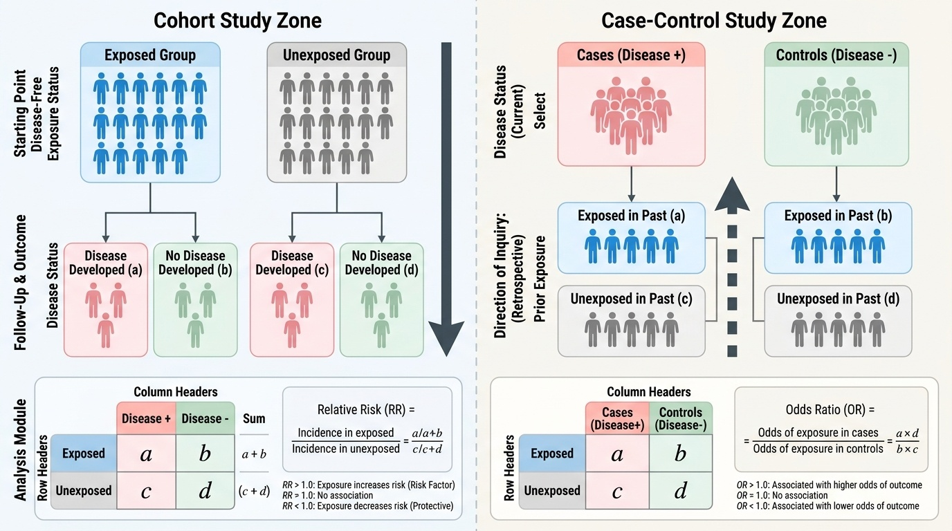
Provided image

Strengths: efficient for rare diseases and long-latency diseases; relatively cheap and fast; can study multiple exposures from a single outcome. Limitations: cannot compute incidence or RR directly (only OR); susceptible to recall bias; selection of appropriate controls is critical and difficult; cannot study rare exposures easily.