Page 2 of 13

CM6.{1-2,4} | CM6.{1-2,4} | Statistical Data Workflow — SDL Guide (Part 2)

Data Collection: Census vs Sampling

Once the research question and variable types are defined, the next decision is HOW to collect the data. The two broad approaches are a census (complete enumeration) and a sample survey. The choice determines the statistical validity of your conclusions and the feasibility of your project.

A census collects data from every member of the population. Advantages: complete picture, no sampling error, useful for small populations. Disadvantages: extremely expensive, time-consuming, logistically difficult for large populations, and subject to response fatigue that reduces data quality. Example: the decennial Census of India enumerates every household — a massive government undertaking that takes years and billions of rupees.

A sample survey collects data from a carefully selected subset of the population. The fundamental requirement is that the sample is representative — it must mirror the characteristics of the population so that findings can be generalised. Representativeness is achieved through probability (random) sampling techniques, which give every member of the population a known, non-zero probability of selection.

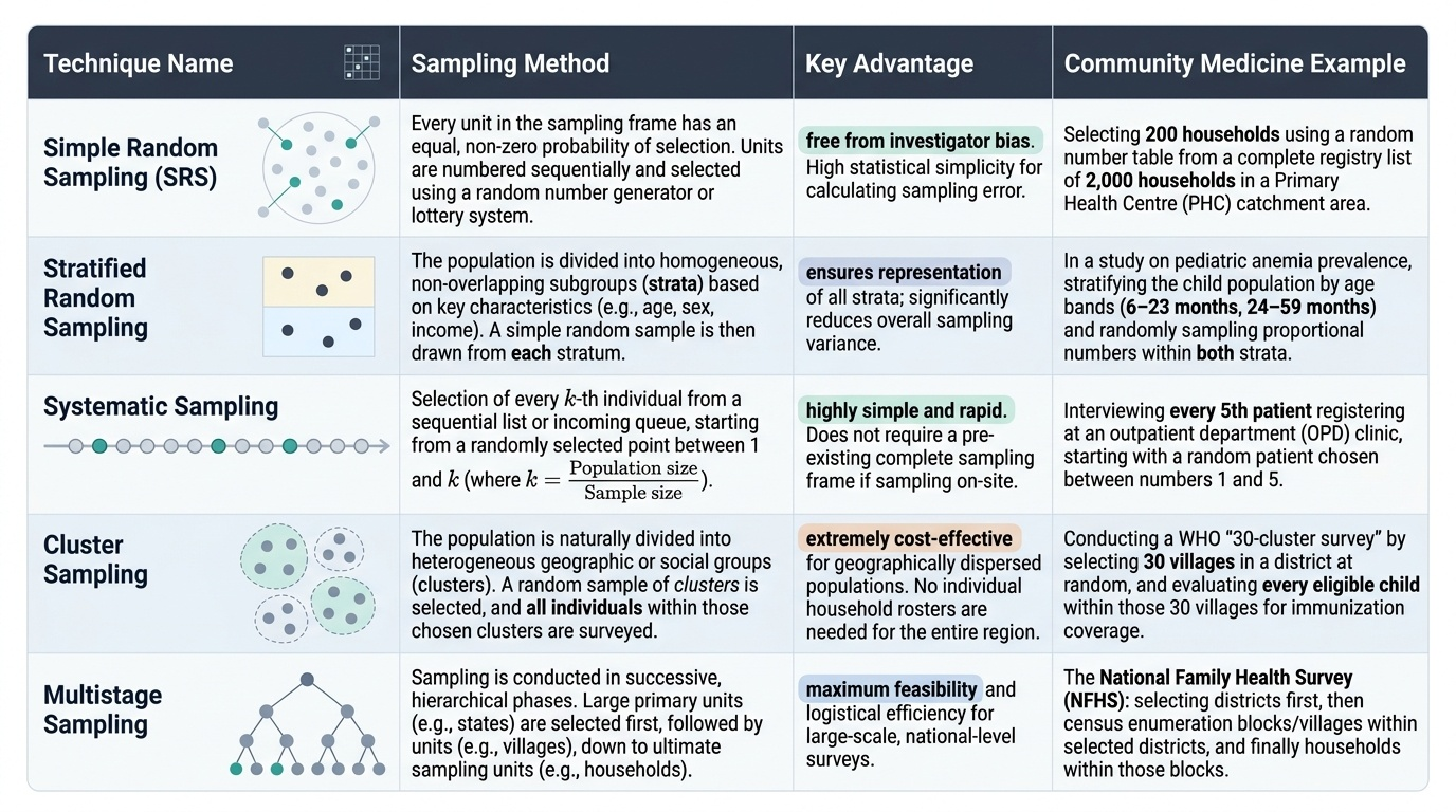
The five major probability sampling techniques (NMC requirement CM6.4):

Provided image

1. Simple Random Sampling (SRS) — Every individual in the sampling frame has an equal probability of selection. Method: number every unit in the sampling frame; select using random number tables or lottery. Example: selecting 200 households from a list of 2,000 registered households in a PHC area. Advantage: free from investigator bias. Limitation: requires a complete sampling frame; impractical for geographically dispersed populations.

1. Stratified Random Sampling — Population is divided into homogeneous subgroups (strata) based on a characteristic related to the outcome (e.g. age, sex, religion, urban/rural). A random sample is drawn from EACH stratum proportional to its size (proportionate) or in fixed numbers (disproportionate/optimal allocation). Example: to study anaemia prevalence, stratify by age group (6–23 months, 24–59 months) and randomly sample within each stratum. Advantage: ensures representation of all strata; reduces variance.

1. Systematic Sampling — Select every k-th unit from a sampling frame after a random start. k = population size / sample size. Example: from a register of 1,000 patients, to select 100: k = 10; pick a random start between 1 and 10, then select every 10th patient. Advantage: simple, evenly distributed; no need for random number tables after the start. Limitation: if the list has a periodic pattern coinciding with k, bias occurs (e.g. if every 10th patient is admitted on Monday).

1. Cluster Sampling — The population is divided into natural clusters (villages, schools, city blocks, PHC areas). Clusters, NOT individuals, are randomly selected; all individuals within selected clusters are surveyed. Example: WHO EPI 30×7 immunisation coverage survey — 30 clusters (usually villages or enumeration blocks) are selected by probability proportional to size, and 7 children are surveyed in each. Advantage: operationally efficient for large, geographically dispersed populations. Limitation: subjects within a cluster tend to be similar (design effect/clustering effect), so the effective sample size is smaller than the actual sample size — standard errors must be adjusted.

1. Multistage Sampling — Sequential application of sampling at multiple levels. Example: National Family Health Survey selects districts (stage 1), then villages/urban blocks within districts (stage 2), then households within villages/blocks (stage 3), then eligible women within households (stage 4). Each stage uses its own probability sampling method. Advantage: practical for national surveys covering hundreds of districts. Most realistic for large-scale community medicine research.

Non-probability sampling methods (convenience, purposive, snowball) are used in qualitative research and pilot studies but cannot support statistical inference about the population — avoid confusing these with the five probability techniques above.

Classification and Presentation of Data

Raw data collected in the field — columns of numbers, tally marks, or questionnaire responses — are unintelligible until organised. Classification imposes order; presentation makes patterns visible. These two steps are the bridge between raw measurement and meaningful interpretation, converting a list of numbers into a picture that reveals distribution, patterns, and outliers. No statistical analysis is valid without first organising the data correctly, and no public-health report is useful without presenting findings in a format that non-statistician administrators can read. This section teaches both skills — and, critically, the rules for choosing the correct graph type for each kind of data.

A well-constructed frequency table is the foundation. It reveals immediately the shape of the distribution — whether data cluster in the middle (bell-shaped), pile up at one extreme (skewed), or spread uniformly. The choice of class intervals matters: too few (e.g. only 3 groups) hide internal variation; too many (e.g. 30 groups for 100 observations) restore the original chaos. A rule of thumb is 5–15 class intervals for most medical datasets. Class boundaries must be non-overlapping and exhaustive (every observation fits into exactly one interval).

Classification: Frequency Distributions

The first step is to arrange raw data into a frequency distribution table: a systematic listing of data values or ranges (class intervals) alongside their frequency of occurrence. For continuous data:
- Choose class intervals that are equal, non-overlapping, and cover the entire range. A rule of thumb is 5–15 class intervals.
- Determine class boundaries carefully (e.g. 10–19 and 20–29, not 10–20 and 20–30, to avoid ambiguity).
- Compute relative frequency (proportion) and cumulative frequency for each interval.

For discrete and nominal data, each value or category has its own frequency row. Tally marks (groups of five) speed up manual counting.

Graphical Presentation

The type of graph must match the type of data — a mismatch gives a misleading picture and is a common exam error:

• Histogram — for continuous data grouped into class intervals. Bars are adjacent (no gaps), and the X-axis is a continuous scale. The area of each bar is proportional to frequency. Example: distribution of diastolic BP readings.
• Frequency Polygon — constructed by connecting the midpoints of the tops of histogram bars. Useful for comparing two frequency distributions on the same graph. Example: comparing age distribution of cases vs controls.
• Bar Chart (Bar Diagram) — for discrete or nominal data. Bars are separated by spaces (reflecting non-continuity of categories). Bars can be simple, multiple (grouped), or component (stacked). Example: incidence of malaria by district, immunisation coverage by vaccine type.
• Pie Chart — circular diagram divided into sectors proportional to each category's percentage. Best for showing composition of a whole. Example: percentage of deaths attributable to different causes.
• Ogive (Cumulative Frequency Curve) — plot of cumulative frequency (or percentage) against class boundaries. Used to read off percentiles and medians graphically.
• Line Diagram — for data collected over time (time-series). X-axis = time; Y-axis = value. Example: weekly malaria cases over 52 weeks.
• Scatter Diagram — for showing the relationship between two continuous variables. Essential for correlation analysis.

A high-yield exam distinction: histogram vs bar chart — histogram: continuous data, no gaps; bar chart: discrete/categorical data, gaps between bars.

Measures of Central Tendency and Dispersion

A frequency distribution tells us where data points lie, but two summary numbers — one measuring the 'centre' (central tendency) and one measuring 'spread' (dispersion) — are needed to communicate the distribution concisely. Together they allow comparison across populations and groups.

Measures of Central Tendency

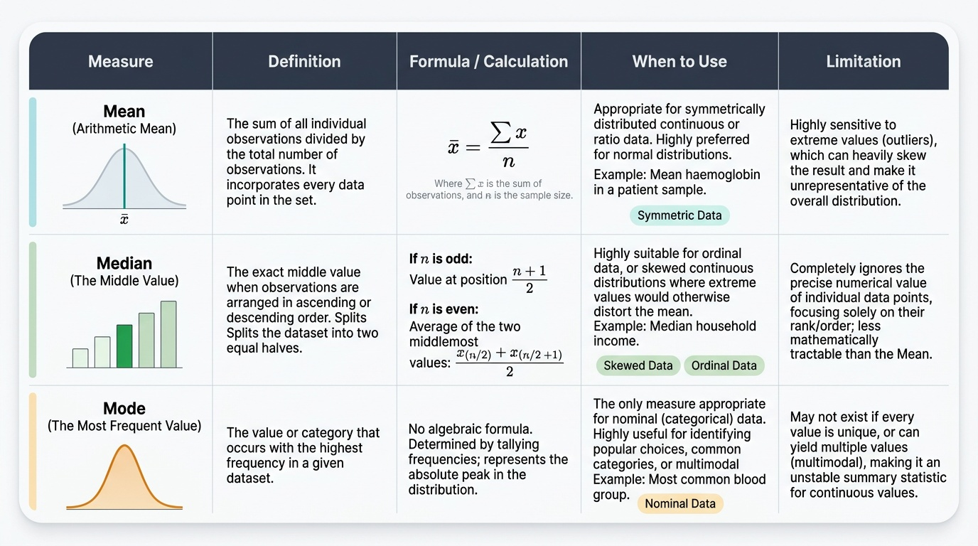
Mean (Arithmetic Mean) — the sum of all observations divided by the number of observations (x̄ = Σx / n). The most mathematically tractable measure; uses every data point. Appropriate for: symmetrically distributed continuous or ratio data. Sensitive to extreme values (outliers). Example: the mean haemoglobin in a sample of 50 women = sum of all 50 Hb values ÷ 50.

Median — the middle value when data are arranged in ascending order. If n is even, the median = average of the two middle values. Appropriate for: ordinal data, or skewed continuous data where outliers distort the mean. Not influenced by extreme values. Example: median household income is more representative than mean income in a community with a few very wealthy families.

Mode — the value (or category) that occurs most frequently. The only appropriate measure for nominal data. A distribution may be unimodal, bimodal, or multimodal. Example: the modal blood group in a clinic population; the most commonly reported symptom in a disease cluster.

Choosing among the three: For normal (bell-shaped) distributions, mean = median = mode and the mean is preferred. For positively skewed distributions (long right tail), mean > median > mode — use the median. For nominal data, use only the mode.

Provided image

Measures of Dispersion

Two datasets can have identical means but very different spreads — dispersion measures capture this variability.

Range — the difference between the maximum and minimum value. Simplest, but uses only two data points and is heavily influenced by outliers. Range alone is insufficient to characterise a distribution.

Variance — the average of the squared deviations from the mean. For a sample: s² = Σ(xᵢ − x̄)² / (n−1). Dividing by (n−1) rather than n gives an unbiased estimate of the population variance (Bessel's correction). Units are the square of the original units (e.g. kg²), making interpretation difficult.

Standard Deviation (SD) — the square root of variance; expressed in the same units as the data. The most commonly used measure of spread for continuous normally distributed data. A small SD means data cluster tightly around the mean; a large SD means wide variability. Example: Hb 11.5 ± 2.3 g/dL means the SD is 2.3 g/dL.

Standard Error of the Mean (SE) — a critically different concept from SD. SE = SD / √n. While SD measures variability WITHIN a sample (how spread out individuals are), SE measures the precision of the sample mean as an estimate of the population mean — i.e., how much the mean would vary across repeated samples. SE decreases as sample size increases. SE is used to construct confidence intervals and conduct significance tests; SD is used to describe the data distribution. Confusing SD and SE is a classic and consequential error.

Coefficient of Variation (CV) — CV = (SD / mean) × 100%. A dimensionless measure that allows comparison of variability across datasets with different units or different means. Example: CV of height (10%) vs CV of income (80%) — tells you income is much more variable relative to its mean.

Interquartile Range (IQR) — Q3 − Q1 (the middle 50% of data). Robust to outliers; used alongside the median for skewed or ordinal data. Presented in box plots.

Percentiles and Quartiles — percentiles divide ranked data into 100 equal parts; quartiles divide into 4. Q1 = 25th percentile, Q2 = 50th percentile (= median), Q3 = 75th percentile. Widely used in growth charts (weight-for-age, height-for-age).